The Pair Correlation Surface Associated to Zeros of Automorphic L-functions

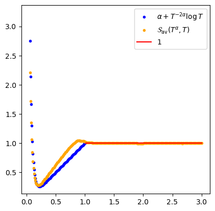
Plots of \(\mathcal{S}_{\mathrm{av},\pi}(T^{m\alpha}, T)\)

As a point of reference, we include a reformulation of a conjecture from Murty and Zaharescu [5] for automorphic \(L\)-functions. Let \(\mathscr{A}_m\) be the set of irreducible cuspidal automorphic representations of representations of \(\mathrm{GL}_m\) over \(\mathbb{Q}\) with unitary central character. This conjecture follows for small \(\alpha\) by the work of Rudnick and Sarnak [7].

Conjecture(Murty and Zaharescu, 2002).

For any \(\pi \in \mathscr{A}_m,\) as \(T \to \infty,\) one has \begin{align*} \mathcal{S}_{\pi,\mathrm{av}}(T^{m\alpha},T) = \begin{cases}|\alpha|+m T^{-2|\alpha| m} \log T(1+o(1))+o(1) & \text { if }|\alpha| \leqslant 1, \\ 1+o(1) & \text { if }|\alpha| \geqslant 1.\end{cases} \end{align*}

From this conjecture, we expect that for \(\alpha\) not too small \(S_{\pi,\mathrm{av}}\) to behave linearly and then flatline for \(|\alpha| \geq 1\). For \(\alpha\) small the denominating term is second term of the first case above. When \(L(s,\pi) = \zeta(s)\) and \(T\) is the millionth zero of \(\zeta\)(\(\approx 600,270\)) this change of main term happens around \(.2\) as seen in the graph. As expected, Montgomery's Theorem and heuristic approximates the behavior of \(S_{\textrm{av}}\) very well [5]. The same can be said for the \(\mathrm{GL}_2\) \(L\)-functions.

Discrete approximations of the Pair Correlation Surface(PCS)

In the box to the right, we present animations of the discrete approximations of the PCS generated from the first million zeros of \(\zeta(s),L(s,\Delta)\)and \(L(s,E).\) In each animation, we take \(.2 \leq |\alpha| \leq 3 \) for smaller \(\alpha\) see the box, Distortion to the PCS.

The animations have three dimensions: the \(\alpha\) dimension, the \(\lambda\) dimension, and the dimension corresponding to the approximation of probability distribution function associated to

\begin{align*} \bigg\{ \frac{\mathcal{S}_{\pi} (T^{m\alpha},T,\frac{1}{2}+\gamma_{\pi})-\mathcal{S}_{\pi,\text{av}}(T^{m \alpha},T)}{\mathcal{S}_{\pi,\text{SD}}(T^{m \alpha},T)}:& |\gamma_{\pi}| \leq T \hspace{1em} \text {and} \hspace{1em} L\Big(\frac{1}{2}+i\gamma_{\pi}\Big) =0 \bigg\} \end{align*}

with \(T\) being the ordinate of the millionth zero of \(L(s,\pi).\) The set above is normalized to have mean zero and standard deviation 1. For each fixed \(\alpha,\) we compute 500 histograms for the set above. We use \(\lambda\) to denote the bin location. For a cleaner presentation, we delete the extreme outliers of this set, which corresponds to one percent of the data. Combining all the \(\alpha\) traces, we create the animations to the left. Examples of the \(\alpha\) traces are displayed in the box The trace of PCS at \(\alpha = 1/2.\)

Finally, we invite the reader to compare these animations to the animation found in the box, The Pair Correlation Surface(PCS).

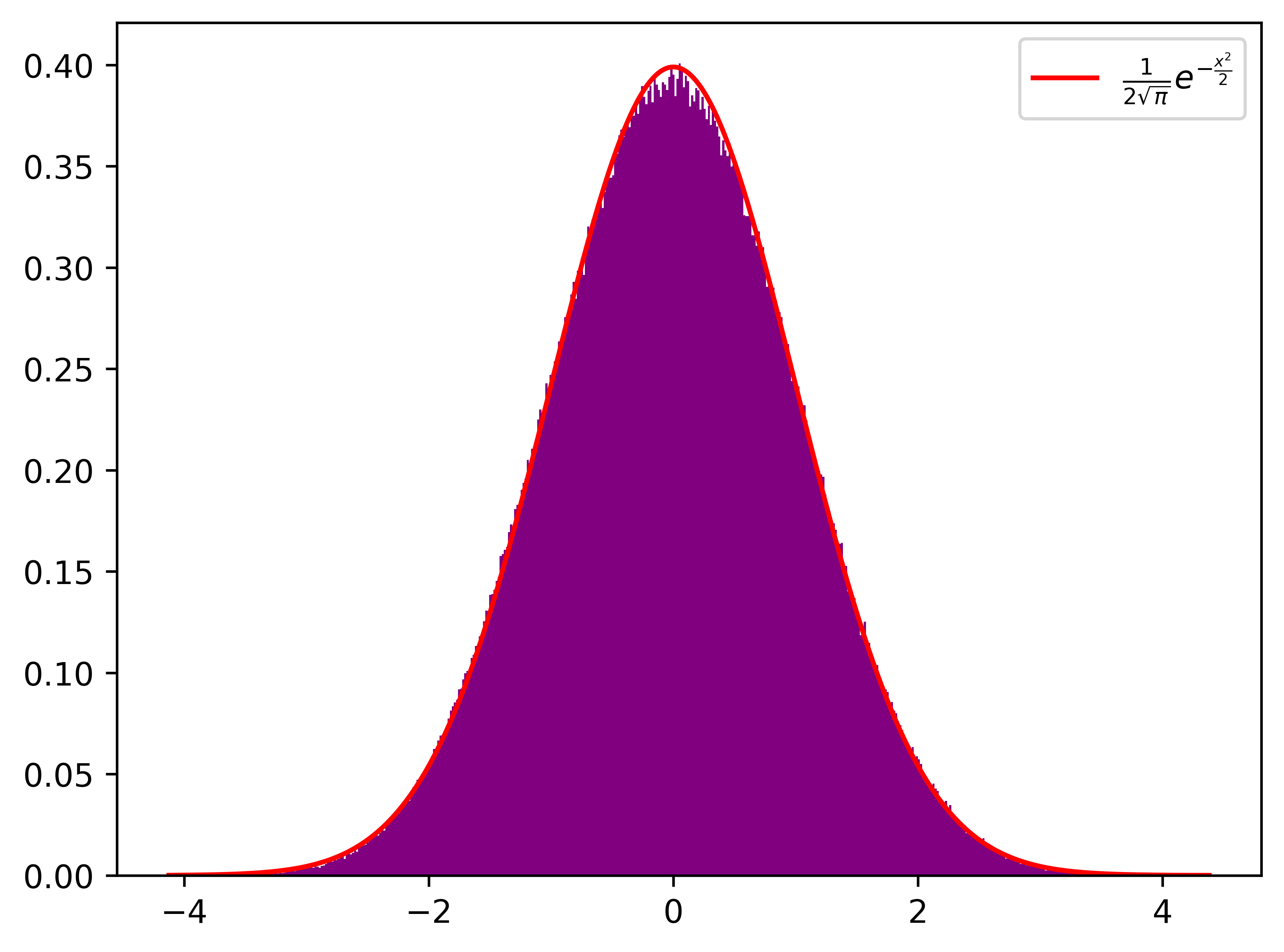
The trace of the PCS at \(\alpha=\frac{1}{2}\)

To the right, are \(\alpha\) traces of the discrete approximations of the PCS when \(\alpha = \frac{1}{2}.\) Explicity, they are the plots of 500 density histograms generated from

\begin{align*} \bigg\{ \frac{\mathcal{S}_{\pi} (T^{m\alpha},T,\frac{1}{2}+\gamma_{\pi})-\mathcal{S}_{\pi,\text{av}}(T^{m \alpha},T)}{\mathcal{S}_{\pi,\text{SD}}(T^{m \alpha},T)}:& |\gamma_{\pi}| \leq T \hspace{1em} \text {and} \hspace{1em} L\Big(\frac{1}{2}+i\gamma_{\pi}\Big) =0 \bigg\} \end{align*}

with \(T\) being the ordinate of the millionth zero of \(L(s,\pi).\) We also plot the gaussian probability distribution function in red.

The Pair Corrrelation Surface (PCS)

In this box, we have an animation of the conjectured PCS for \(|\alpha|\leq 3.\) For the definition of PCS surface associated ot the zeros of \(L(s,\pi)\) see [1, Definition 1.2]

The conjectured Pair Correlation Surface associated to the zeros of \(L(s, \pi)\) is the graph of the function \(g_{\pi} : \mathbb{R}^2 \to \mathbb{R}\) defined by \begin{align}\label{PCS Equation} g_{\pi}(\alpha, \lambda) = \frac{1}{\sqrt{2 \pi}} e^{- \frac{1}{2}\lambda^2}. \end{align} We invite the reader to compare this animation to the ones found in the box Discrete approximations of the PCS.

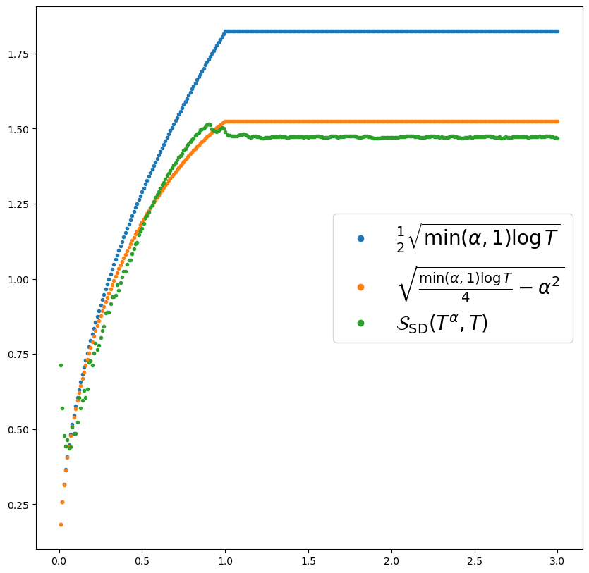
Plots of the standard deviation

In this box, we plot the standard deviations of the \(S_{\pi}(T^{m\alpha},T,\rho_{\pi})\). We denote the standard deviation by \(S_{\pi,SD}(T^{m\alpha},T)\). In consideration of [1, eq. 3.11] and [1, Lemma 3.3], we compare the computed standard deviation to the following estimates \begin{align*} \sqrt{\frac{\min\{1,\alpha\} m \log T}{4}} \end{align*} and \begin{align*} \sqrt{\frac{\min\{1,\alpha\} m \log T}{4}-(\min\{1,\alpha\})^2}. \end{align*} In the last estimate, we add in a lower order term. This inclusion comes from [1, eq. 3.11]. Just like with the averages, we see that the standard deviations flatline after \(\alpha \geq 1.\)

Distortion to the PCS

To the right, we are plotting discrete approximation of the PCS when \(|\alpha|\leq .2\). Namely, we are plotting for each \(\alpha,\) 500 density histograms generated from

\begin{align*} \bigg\{ \frac{\mathcal{S}_{\pi} (T^{m\alpha},T,\frac{1}{2}+\gamma_{\pi})-\mathcal{S}_{\pi,\text{av}}(T^{m \alpha},T)}{\mathcal{S}_{\pi,\text{SD}}(T^{m \alpha},T)}:& |\gamma_{\pi}| \leq T \hspace{1em} \text {and} \hspace{1em} L\Big(\frac{1}{2}+i\gamma_{\pi}\Big) =0 \bigg\} \end{align*}

As \(\alpha\) approaches \(0\), we see that in the graph the distribution is looking less normal, in fact, it is even becoming less symmetric(see the Tables tab for the values of some odd moments). This is a natural extension of the change of main term seen in the average, Plots of \(\mathcal{S}_{\mathrm{av},\pi}(T^{m\alpha}, T)\)